OEE Calculation example
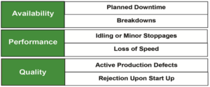
OEE is formulated as a function of a number of mutually exclusive components, such as availability efficiency, performance efficiency, and quality efficiency in order to quantify various types of productivity losses.
During the design of the production system the use of intrinsic performance index for the sizing of each equipment although wrong could seem the only rational approach for the design. By the way, this approach don’t consider the interaction between the stations. Someone can argue that to make independent each station from the other stations through the buffer would simplify the design and increase the availability. Still, the interposition of a buffer between two or more station may not be possible for several reason. Most relevant are:
- logistic (space unavailability, huge size of the product, compact plant layout, etc.);
- economic (the creation of stock amid each couple of station increase the WIP and consequently interest on current assets);
- performance;
- product features (buffer increase cross times, critical for perishable products);
In our model we will show how a production system can be defined considering availability, performance and quality efficiency (5),(6), (7) of each station along with their interactions. The method embraces a set of hints and suggestions (best practices) that lead designers in handle interactions and losses propagation with the aim to rise the expected performance of the system. Furthermore, through the development of a simulation model of a real production system for the electrical cable production we provide students with a clear understanding of how time-losses propagate in a real manufacturing system.
The design process of a new production system should always include the simulation of the identified solution, since the simulation provides designer with a holistic understanding of the system. In this sense in this paragraph we provide a method where the design of a production system is an iterative process: the simulation output is the input of a successive design step, until the designed system meet the expected performance and performance are validated by simulation. Each loss will be firstly described referring to a single equipment, than its effect will be analyzed considering the whole system, also throughout the support of simulation tools.
Set Up Availability
Availability losses due to set up and changeover must be considered during the design of the plant. In accordance with the production mix, the number of set-up generally results as a trade-off between the set up costs (due to loss of availability + substituted tools, etc.) and the warehouse cost.
During the design phase some relevant consideration connected with set-up time losses should be considered. A production line is composed of n stations. The same line can usually produce more than one product type.
Depending on the difference between different product types a changeover in one or more stations of the line can be required. Usually, the more negligible the differences between the products, the lower the number of equipments subjected to set up (e.g. it is sufficient the set up only of the label machine to change the labels of a product depending on the destination country). In a given line of n equipments, if a set up is requested in station i, loss availability can interest only the single equipment I or the whole production line, depending on the buffer presence, their location and dimension:
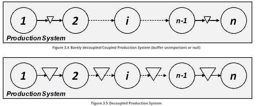
- If buffers are not present, the set up of station i implies the stop of the whole line ( Figure 3.4 ). This is a typical configuration of flow shop process realized by one or more production line as food, beverages, pharmaceutical packaging,….
- If buffers are present (before and beyond the station i) and their size is sufficient to decouple the station i by the other i-1 and i+1 station during the whole set up, the line continues to work regularly ( Figure 3.5 ).
Hence, the buffer design plays a key role in the phenomena of losses propagation throughout the line not only for set-up losses, but also for other availability losses and performance losses as well. The degree of propagation ranges according to the buffer size amid zero (total dependence-maximum propagation) and maximum buffer size (total independence-no propagation). It will be debated in the following (§ 3.5.3), when considering the performance losses, although the same principles can be applied to avoid propagation of minor set up losses (mostly for short set-up/changeover, like adjustment and calibrations).
Maintenance Availability
The availability of an equipment is defined as:
![]()
The availability of the whole production system can be defined similarly. Nevertheless it depends upon the equipment configurations. Operations Manager, through the choice of equipment configurations can increase the maintenance availability. This is a design decision, since different equipments must be bought and installed according to desired availability level. The choice of the configuration usually results as a trade-off between equipment costs and system availability. The two main equipment configuration (not-redundant system, redundant system) are debated in the following.
Not redundant system
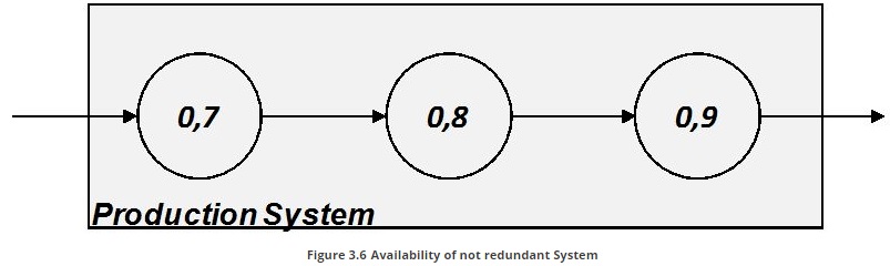
When a system is composed of non redundant equipment, each station produces only if the equipment is working.
Hence if we consider a line of n equipment connected as a series we have that the downtime of each equipment causes the downtime of the whole system.

The availability of system composed of a series of equipment is always lower than the availability of each equipment ( Figure 3.6 ).
Total redundant system
Oppositely, to avoid failure propagation amid stations, designer can set the line with a total redundancy of a given equipment. In this case only the contemporaneous downtime of both equipments causes the downtime of the whole system.
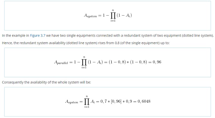
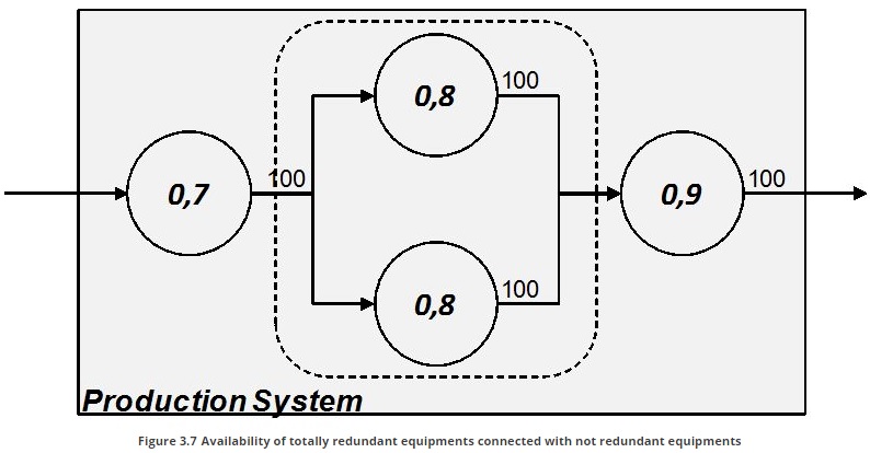
To achieve an higher level of availability it has been necessary to buy two identical equipments (double cost). Hence, the higher value of availability of the system should be worth economically.
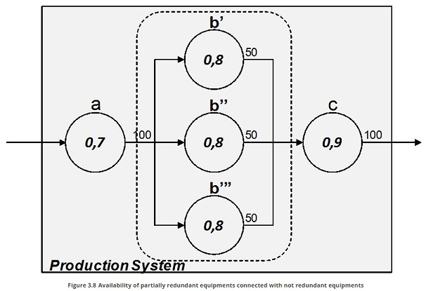
Partial redundancy
An intermediate solution can be the partial redundancy of an equipment. This is named K/n system, where n is the total number of equipment of the parallel system and k is the minimum number of the nequipment that must work properly to ensure the throughput is produced. The Figure 3.8 shows an example.
The capacity of equipment b’, b’’ and b’’’ is 50 pieces in the referral time unit. If the three systems must ensure a throughput of 100 pieces, it is at least necessary that k=2 of the n=3 equipment produce 50 pieces. The Table 3.7 shows the configuration states which ensure the output is produced and the relative probability that each state manifests.
|
b’ |
b’’ |
b’’’ |
Probability of occurrance |
[*100] |
|---|---|---|---|---|
|
UP |
UP |
UP |
0,8*0,8*0,8 |
0,512 |
|
UP |
UP |
DOWN |
0,8*0,8*(1-0,8) |
0,128 |
|
UP |
DOWN |
UP |
0,8*(1-0,8)*0,8 |
0,128 |
|
DOWN |
UP |
UP |
(1-0,8)*0,8*0,8 |
0,128 |
|
Total Availability |
0,896 |
|||
In this example all equipments b have the same reliability (0,8), hence the probability the system of three equipment ensure the output should have been calculated, without the state analysis configuration ( Table 3.7 ), through the binomial distribution:
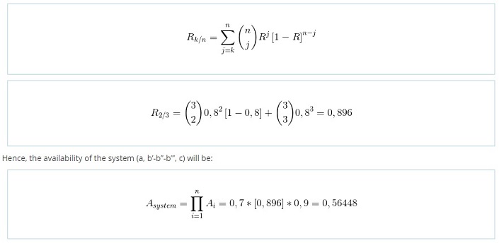
In this case the investment in redundancy is lower than the previous. It is clear how the choice of the level of availability is a trade-off between fix-cost (due to equipment investment) and lack of availability.
In all the cases we considered the buffer as null.
When reliability of the equipments (b in our example) the binomial distribution (16) is not applicable, therefore the state analysis configuration ( Table 3.7 ) is required.
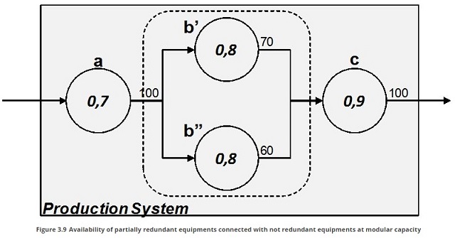
Redundancy with modular capacity
Another configuration is possible.
The production system can be designed as composed of two equipment which singular capacity is lower than the requested but which sum is higher. In this case if it is possible to modulate the production capacity of previous and successive stations the expected throughput will be higher than the output of a singular equipment.
Considering the example in Figure 3.9 when b’ and b’’ are both up the throughput of the subsystem b’-b’’ is 100, since capacity of a and c is 100. Supposing that capacity of a and c is modular, when b’ is down the subsystem can produce 60 pieces in the time unit. Similarly, when b’’ is down the subsystem can produce 70. Hence, the expected amount of pieces produced by b’-b’’ is 84,8 pieces ( Table 3.8 ).
When considering the whole system if either a or c are down the system cannot produce. Hence, the expected throughput in the considered time unit must be reduced of the availability of the two equipments:
|
b’ |
b’’ |
Maximum Throughput |
Probability of occurrence |
[*100] |
Expected Pieces Produced |
|---|---|---|---|---|---|
|
UP |
UP |
100 |
0,8*0,8 |
0,64 |
64 |
|
UP |
DOWN |
70 |
0,8*(1-0,8) |
0,16 |
11,2 |
|
DOWN |
UP |
60 |
(1-0,8)*0,8 |
0,16 |
9,6 |
|
Expected number of Pieces Produced |
84,8 |
||||
Minor Stoppages and Speed Reduction
OEE theory includes in performance losses both the cycle time slowdown and minor stoppages. Also time losses of this category propagate, as stated before, throughout the whole production process.
A first type of performance losses propagation is due to the propagation of minor stoppages and reduced speed among machines in series system. From theoretical point of view, between two machines with the same cycle time – and without buffer, minor stoppage and reduced speed propagate completely like as major stoppage. Obviously just a little buffer can mitigate the propagation.
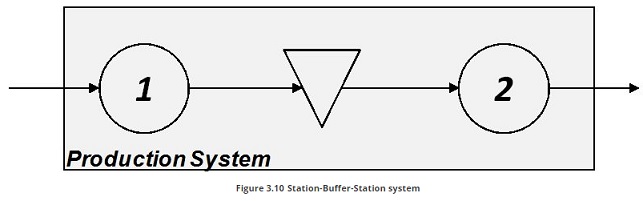
Several models to study the role of buffers in avoiding the propagation of performance losses are available in Buffer Design for Availability literature. The problem is of scientific relevance, since the lack of opportune buffer between the two stations can indeed affect dramatically the availability of the whole system. To briefly introduce this problem we refer to a production system composed of two consecutive equipments (or stations) with an interposed buffer ( Figure 3.10 ).
Under the likely hypothesis that the ideal cycle times of the two stations are identical, the variability of speed that affect the stations is not necessarily of the same magnitude, due to its dependence on several factors. Furthermore Performance index is an average of the Tt, therefore a same machine can sometimes perform at a reduced speed and sometimes an highest speed . The presence of this effect in two consecutive equipments can be mutually compensate or add up. Once again, within the propagation analysis for production system design, the role of buffer is dramatically important.
When buffer size is null the system is in series. Hence, as for availability, speed losses of each equipment affect the performance of the whole system:
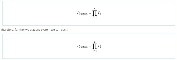
But when the buffer is properly designed, it doesn’t allow the minor stoppages and speed losses to propagate from a station to another. We define this Buffer size as Bmax. When, in a production system of n stations, given any couple of consecutive station, the interposed buffer size is Bmax (calculated on the two specific couple of stations), then we have:
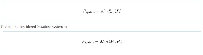
Hence, the extent of the propagation of performance losses depends on the buffer size (j) that is interposed between the two stations. Generally, a bigger buffer increases the performance of the system, since it increases the decoupling degree between two consecutive stations, up to j=Bmax is achieved (j =0,..,Bmax).
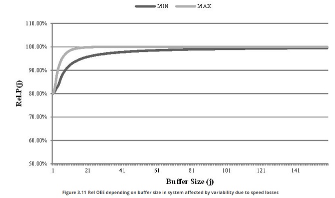
We can therefore introduce the parameter
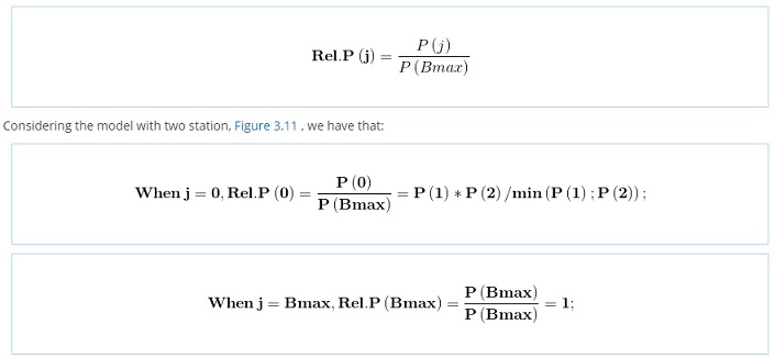
Figure 3.11 shows the trend of Rel.P(j) depending on the buffer size (j), when the performance rate of each station is modeled with an exponential distribution5 in a flow shop environment. The two curves represent the minimum and the maximum simulation results. All the others simulation results are included between these two curves. Maximum curve represents the configuration with the lowest difference in performance index between the two stations, the minimum the configuration with the highest difference.
By analyzing the Figure 3.11 it is clear how an inopportune buffer size affect the performance of the line and how increase in buffer size allows to obtain improve in production line OEE. By the way, once achieved an opportune buffer size no improvement derives from a further increase in buffer. These considerations of Performance index trend are fundamental for an effective design of a production system.
Quality Losses
In this paragraph we analyze how quality losses propagate in the system and if it is possible to assess the effect of quality control on OEE and OTE.
First of all we have to consider that quality rate for a station is usually calculated considering only the time spent for the manufacturing of products that have been rejected in the same station. This traditional approach focuses on stations that cause defects but doesn’t allow to point out completely the effect of the machine defectiveness on the system. In order to do so, the total time wasted by a station due to quality losses should include even the time spent for manufacturing of good products that will be rejected for defectiveness caused by other stations. In this sense quality losses depends on where scraps are identified and rejected. For example, scraps in the last station should be considered loss of time for the upstream station to estimate the real impact of the loss on the system and to estimate the theoretical production capacity needed in the upstream station. In conclusion the authors propose to calculate quality rate for a station considering as quality loss all time spent to manufacture products that will not complete the whole process successfully.
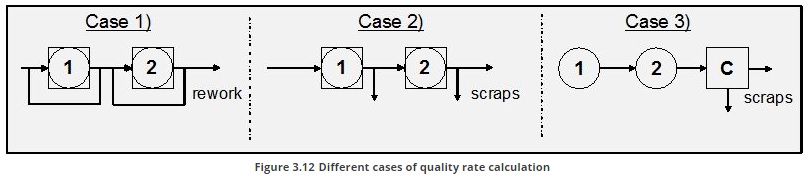
From a theoretical point of view we could consider the following case for calculation of quality rate of a station that depends on types of rejection (scraps or rework) and on quality controls positioning. If we consider two stations with an assigned defectiveness Sj and each station reworks its scraps with a rework cycle time equal to theoretical cycle time, quality rate could be formulate as shown in case 1 in Figure 3.12. Each station will have quality losses (time spent to rework products) due its own defectiveness. If we consider two stations with an assigned defectiveness Sj and a quality control station at downstream each station, quality rate could be formulate as shown in case 2 in Figure 3.12. The station 1, that is the upstream station, will have quality losses (time spent to work products that will be discarded) due to its own and station 2 defectiveness. If we consider two stations with an assigned defectiveness Sj and quality control station is only at the end of the line, quality rate quality rate could be formulate as shown in case 3 in Figure 3.12. In this case both stations will have quality losses due to the propagation of defectiveness in the line. Case 2 and 3 point out that quality losses could be not simple to evaluate if we consider a long process both in design and management of system. In particular in the quality rate of station 1 we consider time lost for reject in the station 2.
Finally, it is important to highlight the different role that the quality efficiency plays during the design phase and the production.
When the system is producing, Operations Manager focuses his attention on the causes of the delectability with the aim to reduce it. When it is to design the production system, Operations Manager focuses on the expected quality efficiency of each station, on the location of quality control, on the process (rework or scraps) to identify the correct number of equipments or station for each activity of the process.
In this sense, the analysis is vertical during the production phase, but it follows the whole process during the design ( Figure 3.13 ).